2) Extraction of the intensity profile
- Open the RAW file in a relevant
software (I use AstroArt, but others may do the job).
- Extract the red channel.
- Check whether there is no
saturation in the fringe system (otherwise use a shorter exposure time).
- Export the intensity profile
along the horizontal line passing though the center of the interference fringe
system in .txt file (or other format).
Notes:
- If the 14-bit RAW files can't be read
directly by the processing software, they can be converted to
16-bit files using Adobe DNG converter.
- The profile of the fringes in red
channel is analysed along the horizontal diameter (X axis) or any
other slice passing through the center of the fringe system.
- If the S/N of the profile is low (i.e. noisy):
- A 20-pixel high slice is cropped from the image.
- In this cropped image, the curvature of the fringes is negligeable,
allowing to average the columns (Y axis) in order to increase the S/N.
- For example :
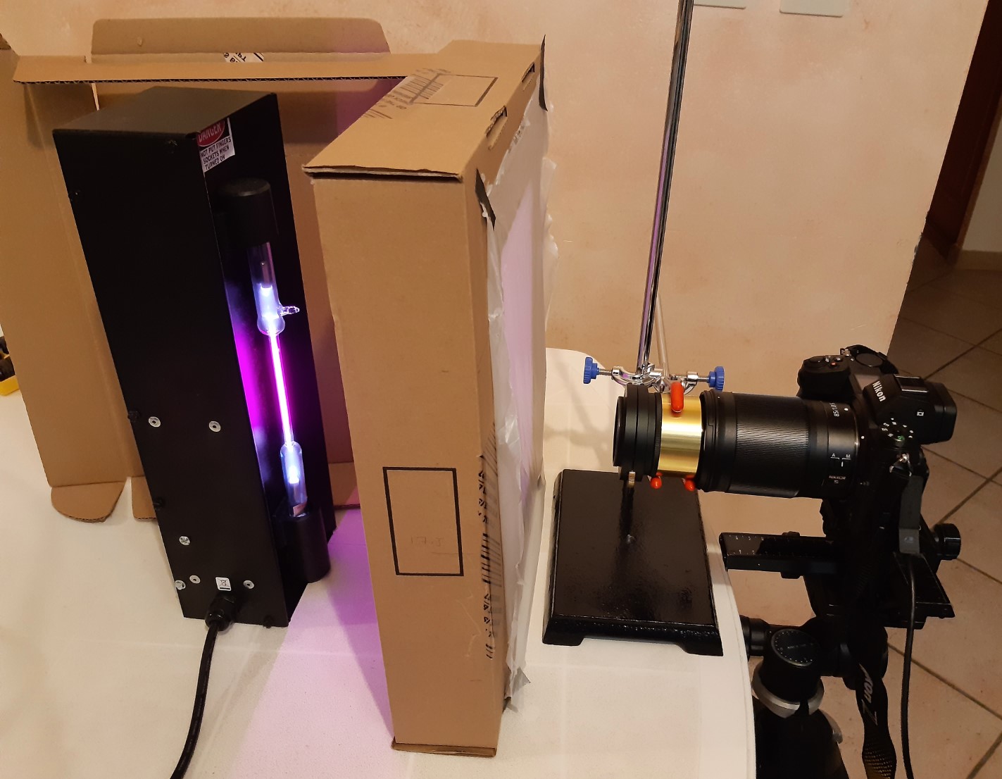
Coronado SM III 60 mm (tilt) - Nikon Z6 with 85 mm S f/1.8 lens at f/1.8 - 100 ISO - 1/2s - 14 bit acquisition - RAW mode - Red channel.
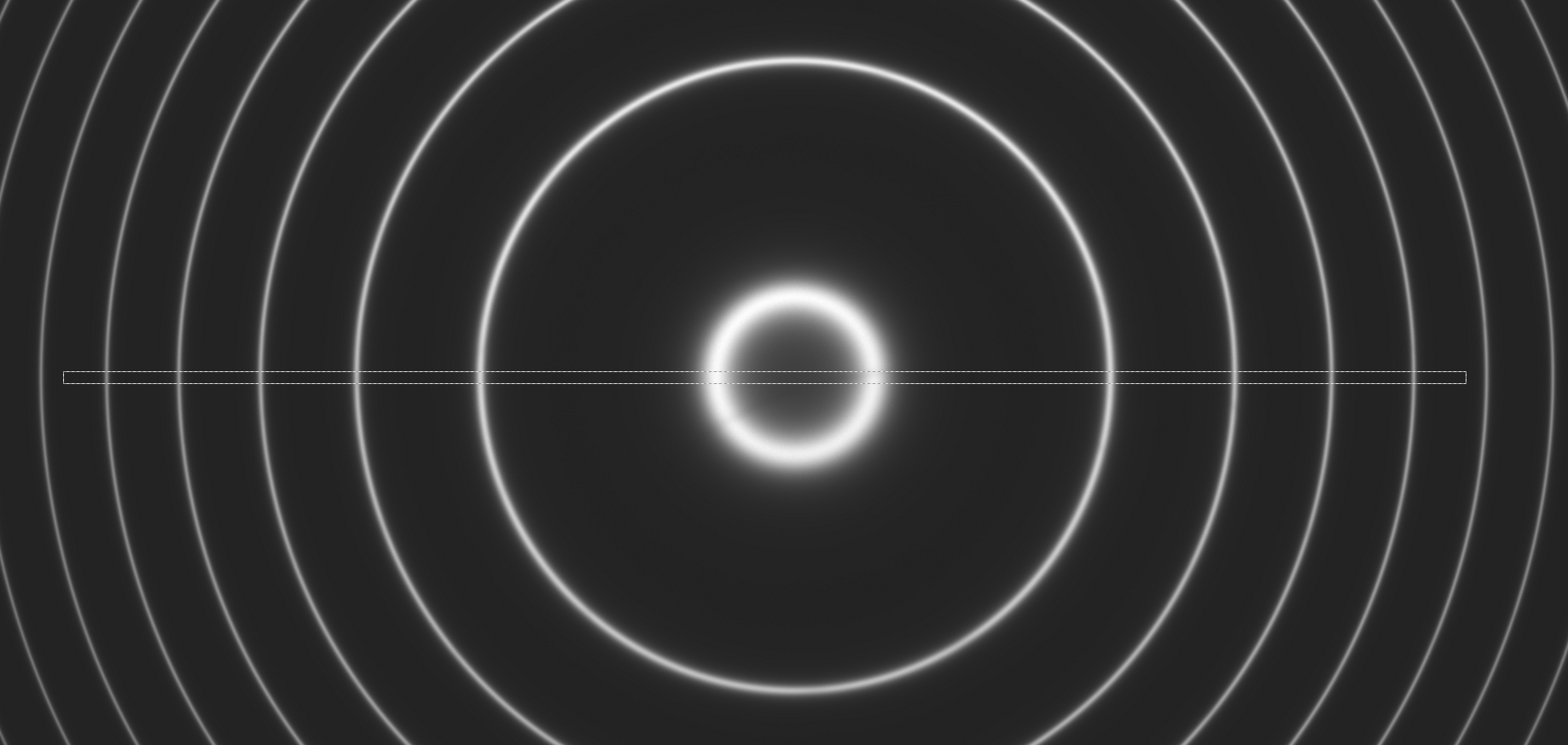
Cropping
a slice of fringes along the horizontal diameter of the etalon.
Note the central dip due to the CWL (red) offset at normal
incidence.
-
- Export the intensity profile
along the horizontal line passing though the center of the interference fringe
system in .txt file (or other format).
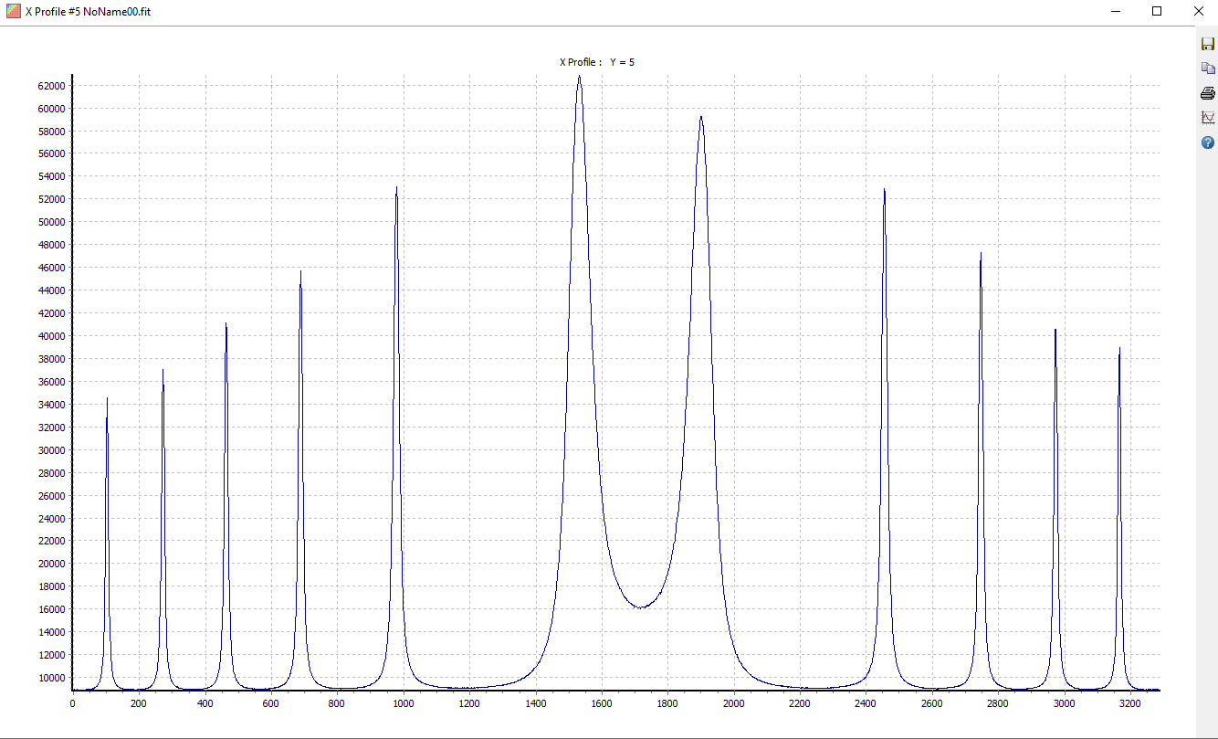
SM III 60 mm (tilt) - Nikon 85 mm f/1.8 S at f/1.8 - 100 ISO - 1/2s.
X profile along the 12 fringes central fringes.
The principle is to measure the
position (X) and the FWHM of each fringe.
For
this, a Voigt function (+
constant) is curved-fitted to each fringe. The constant is used to
account for the offset of the camera. The result of the curve fit is
the
estimation of the position of each peak (X) and of the associated FWHM.
To do this, I use Fityk
freeware:
https://fityk.nieto.pl
- Measured data can be exported (menu Functions/Export Peaks
Parameters), to be used for calculation.
- Some part of the work with Fityk can be probably scripted (see Fityk
website).
o
The CWL of the etalon is
calculated based on the radius of the central ring (if any):
d CWL = i^2/n^2,
where d CWL is in A, i in degrees, n
is the index of the gap (1 for air, about 1.6 for mica).
The radius of this central
ring is not measured by curve-fitting (its profile is not a Voigt), but just by
measuring the X position of the peak. This is accurate enough in general. A more accurate method is described latter on.
Notes:
- If the etalon is reasonably good, the fringe profile should be a Lorenztian function.
- If the etalon is not uniform etalon an/or specially bad,
the fringe profile may be a Voigt function, or even worse a non
symetrical Lorentzian or Voigt function.
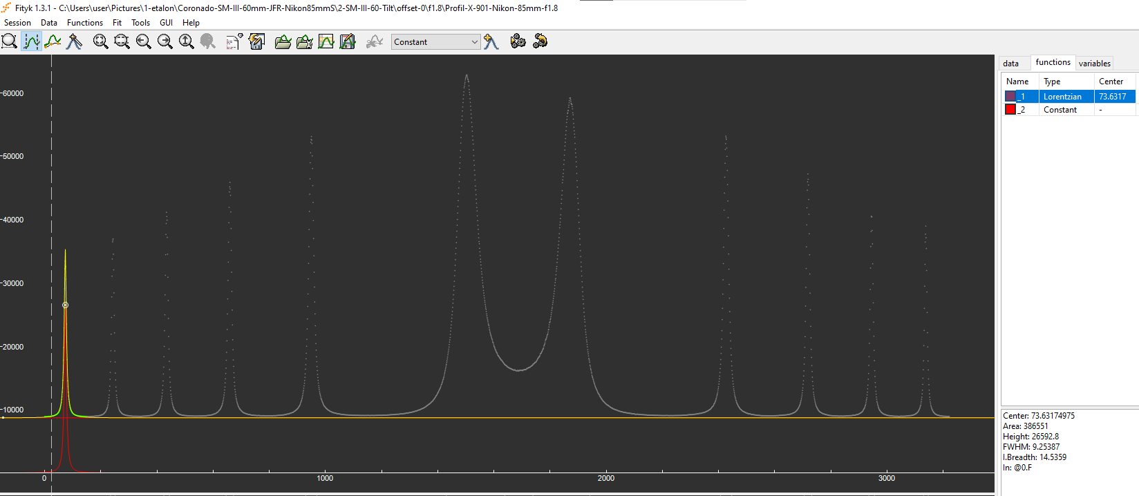
Fitting
a Lorentzian + constant function to fringe #1 Fityk. The
FWHM (9.2 pixel) and center (X= 73.6 pixel) of the Lorentzian is
extracted.
6) Calculation of the CWL, FWHM, FSR and air-gap using the spread sheet
The spread sheet implements the
calculations established by François Rouvières.
o
Input data (red color on yellow
cell):-
- X position and FWHM of each fringe, left and right (measuring five
different fringes is good enough).
- X position, left and right of the central ring (for calculation of
the CWL).
- Pixel size (microns) and focal length of the camera lens (mm): for
calculation of the image scale in degree/pixel.
- Cavity index (n=1 for air).
- Wavelength of Ha (A).
o
Output data:
- FWHM, CWL, FSR, gap.
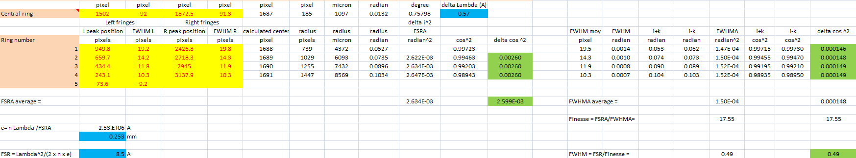
The following extract gives an example of calculation.
(1) On the left side, calculation of the FSR:
- red color in yellow cells: measurements of FWHM and position of 6 fringes (left) and 5 fringes (right)
- calculation of fringe centers: used for checking consistency of input data,
- for each fringe: radius of the fringe = 1/2 diameter
- for each fringe, calculation of the radius of the fringe i in radian (conversion pixel -> micron -> radian)
- for each fringe, calculation of cos^2 (i) (see explanations in the pdf)
- for each couple of sucessive fringes n,
n+1, calculation of cos^2 (i) fringe (n+1) - cos^2(i) fringe (n)
=> this value should be very close to constant (this
is a way to check the accuracy of the measurements) =>
take average value over 3 couple of fringes => result is used
to calculate the FSR in Angstrom : 8.5 A.
(2) On the right side, calculation of finesse and FWHM:
- for each fringe, calculation of the average value of the FWHM of the fringe in pixel (left/ right), conversion in radian,
- for each fringe, calculation of angles i+k, i-k (see explanations in the pdf).
- for each fringe, calculation of FWHMA in radian^2,
- for each fringe, calculation of delta cos^2 (see
explanations in the pdf) => this value should be very close to constant => take
average value over 4 fringes => result is used to calculate the
finesse (=17.55), and FWHM = FSR/ Finesse.
Example of spreadsheet.
Consistency checks and first look at etalon non-uniformity:
- A difference between FWHM L and FWHM R could be an indication of etalon non-uniformity or wrong setup (poor lens quality).
- Another indicatio
n of
non uniformity of an etalon is a bad curve-fit: non symmetrical profile.
- The column "calculated center" should show about the same value, otherwise there is something wrong with the measurements.
- The first column "delta cos 2" (0.00260, etc.) should give fairly
similar results, otherwise something is wrong with the
measurements.
- The second column "delta cos 2" (0.0000146, 0.0000148, etc.) is very
sensitive to the accuracy of focus and optical quality of the
lens.
If some data do not seem accurate enough, they could be excluded from
the calculation of the average FWHMA.
- However, it is better to measure four of
five fringes. This allows a better check of the consistency of the measurement between succesive fringes.
- A difference between FWHM L and FWHM R
could be an indication of etalon non-uniformity or wrong setup (poor lens
quality).
- Another indication of non uniformity of
an etalon is a bad curve-fit: non symmetrical profile.
- The column "calculated center"
should show about the same value for all fringes, otherwise there is something
wrong with the measurements.
- The first column "delta cos 2"
(0.00260, etc.) should give fairly similar results, otherwise something is
wrong with the measurements.
- The second column "delta cos 2"
(0.0000146, 0.0000148, etc.) is very sensitive to the accuracy of focus
and optical quality of the lens. If some data do not seem accurate enough, they
could be excluded from the calculation of the average FWHMA.
- However, it is better to measure four of
five fringes. This allows to better check the consistency of the measurement
between fringes.
7) Correction to be applied to account for the FWHM of the hydrogen lamp
The
method uses a hydrogen lamp as a light source. As the Ha lamp is not perfectly
monochromatic, the measured FWHM is the convolution of the FWHM of the etalon
and the FWHM of the hydrogen lamp.
(FWHM
measured)
2 =(FWHM
etalon)
2 + (FWHM
lamp)
2
Given that the FWHM of the lamp was measured to be 0.263 A (
see more info here), the relation between the measured FWHM and the actual FWHM is :
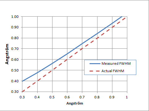
Comparison between measurements using the spectroscope and using the
hydrogen lamp show reliability of results obtained with the hydrogen
lamp down to 0.3 A etalons. However, and to be on the safe side,
it is preferable to keep with the measured (and not deconvoluated)
value when it is lower than 0.35 A.
Accurate measurement of delta CWL
In the method described
above, the delta CWL (at normal incidence) is calculated on the basis
of the diameter of the innermost diffraction ring. This can pose two
practical challenges:
a) Given that the transmission profile is not symetrical,
there is some incertainty in the measurement of the position of the
transmssion peak. Furthermore, the profile it is not a Lorentz nor a
Voigt, so curve fitting - though possible - requires a more elaborate
reference function.
b) When the delta CWL is small, the "innermost ring"
actually merges into the central inteference pattern, and no
measurement is possible.
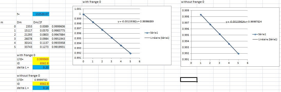
In order to get a more robust and accurate measurement of
the delta CWL, it is better to use the following approach based on a
linear regression on the diameter of the interference rings.
Theoritical grounds by François Rouvière:
delta_CWL.pdf
Formula (6) page 3 is used for the linear regression and
calculate the delta CWL. Note that formula (5) is not accurate enough
because the angles measured are not small enough.
Spread sheet example:
An example of calculation is provided in this spread sheet:
H-lamp-etalon-CWLb.xlsx
Calculation of the CWL is done in columns AC to AF.
NB : in the spreadsheet, two linear regressions are done:
- one including fringe #0,
- one excluding fringe #0.
As the diameter of fringe #0 is not measured by curve-fitting, but only
by direct measurement of the position of its transmission peak, it can
be argued that its measurement is less accurate than the other fringes.
This would suggest not including this measurement in the regression.
However, making both calculations (with and without fringe #0) is
probably informative of the level of accuracy of the measurement of the
delta CWL.
Area of the etalon sampled
The area sampled (i.e. measured) on the etalon is determined by the diameter of the aperture stop of the
camera lens (and also by vignetting due to the
etalon barrel and lens combination). For example, an 85 mm f/1.8 lens samples an area
of (approximately) 46.1 mm in diameter on the etalon, while the same lens at f/8 samples an area less than 10.6 mm.
- An easy way to understand this is as follows :
- The fringe system is at the infinite.
- The size of each fringe on the camera sensor depends on
its angular diameter and on the focal length of the lens (just like the
size of any celestial object).
- The light beam coming from any point of a given fringe
is a collimated beam intercepting the whole surface of the etalon
(except vigneting due to the etalon barrel).
- Accordingly, the size of the area sampled on the
etalon is determined by the size of the aperture stop of the camera
lens (to an approximation, see bottom of the page).
- In a perfect world, and in order to sample the entire
surface of the etalon in a single shot and estimate the average FWHM
and
FSR over the full aperture of the etalon, we should use a lens whose
aperture is similar to the aperture of the etalon. This is an issue because usually lens have a poorer optical quality at
full aperture.
- Otherwise, measurements made with a lens with a
small aperture should be properly integrated over the whole
aperture of the etalon to estimate the FWHM at full aperture..
- The farther the camera (or the eye) from the etalon the lower
the number of fringes is seen (the angular diameter of the fringes is
unchanged, while the angular diameter of the etalon and central
spacer decreases). This does not change thes size of the area sampled
on the etalon.
Local or full-aperture FWHM: what is the most relevant?
The FWHM and CWL of an etalon may vary locally depending on the area sampled on the etalon.
(a) When the etalon is placed in front of the aperture of the telescope:
- All parts of the etalon contribute equally to the quality (i.e.
contrast) of the image. Accordingly, the relevant value to qualify the
etalon performance is the FWHM (and CWL) integrated over the full
aperture of the etalon, and not the local values of FWHM and CWL.
- However, the mapping of the local values of FWHM and CWL can still be
used to calculate the average (or integrated) values over the full
aperture of the etalon. The integration of the FWHM acrossf the full
aperture of the etalon
is correct only if it takes into account both the local values of FWHM and CWL.
- For example, let's consider an etalon whose local values of FWHM are
all 0.3 A, but whose CWL changes dramatically of +/1 A from one area
sampled to the other. If we calculate the average FWHM over
the full aperture of the etalon only from the local FWHM value
statistics, then the result (0.3 A) is wrong, because of
the strong variation of CWL over the aperture. In fact, a correct
calculation should include both FWHM and CWL
statistics.
(b) For an etalon placed in the rear position:
- Let's assume an observation of the Sun with a 2 m focal length
telescope. The diameter of the solar disk at the focal plane is about 2
cm.
- All the area of the etalon within this central 2 cm diameter contribute equally to the contrast of the image.
- Accordingly, the relevant value for the observation is again the average
(or integrated) values of FWHM and CWL, and not the local values.
Accuracy of the measurement
The accuracy of measurement on :
- The quality of the lens used. The FWHM of the lens can be measured
over the field of view and at various f-numbers using CCD inpector.
See various examples here.
- The accuracy of the focal length of the lens. The focal length can be measured using
Astrometry.net
- The accuracy of the focusing.
- The good sampling of the fringe profile in order to get a good
estimate for the curve fitting. To be on the safe side, the FWHM of the
fringe should be greater than 10 pixels.
Measuring air-spaced etalons is much easier than measuring mica-spaced etalons because:
- transmission is much higher (>60%) versus a few percent,
which means better S/N in fringe profiles because lower ISO
can be used,
- smaller FSR (typically 10-12 A versus 20-30 A for mica-spaced
etalons) and refractive index (1 instead of about 1.6), meaning a
larger number of fringes can be measured (more than 5 versus 2 or 3 at
most for mica-spaced etalons),
- the 2nd and 3rd interference fringes of mica-spaced etalons are very
faint, so it is necessary to surexpose massively to detect them,
- for some reason (polarizers not properly aligned ?), it happends that
the fringes of mica-spaced etalons tends to be less symetrical than the
fringes of air-spaced etalons.
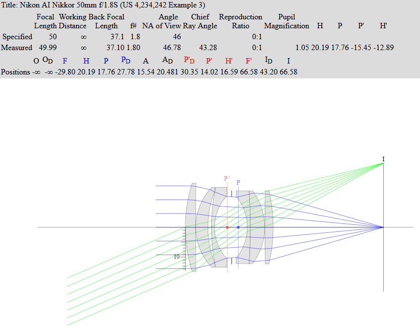
Additional note on the size of area actually sampled on the etalon due to camera lens vigneting effect:
These ray-tracing for Nikon 50 mm f/1.8 are from :
https://www.photonstophotos.net
Nikon 50 mm f/1.8 at f/1.8 - The entrance pupil (Pd in blue) is 27.78 mm.
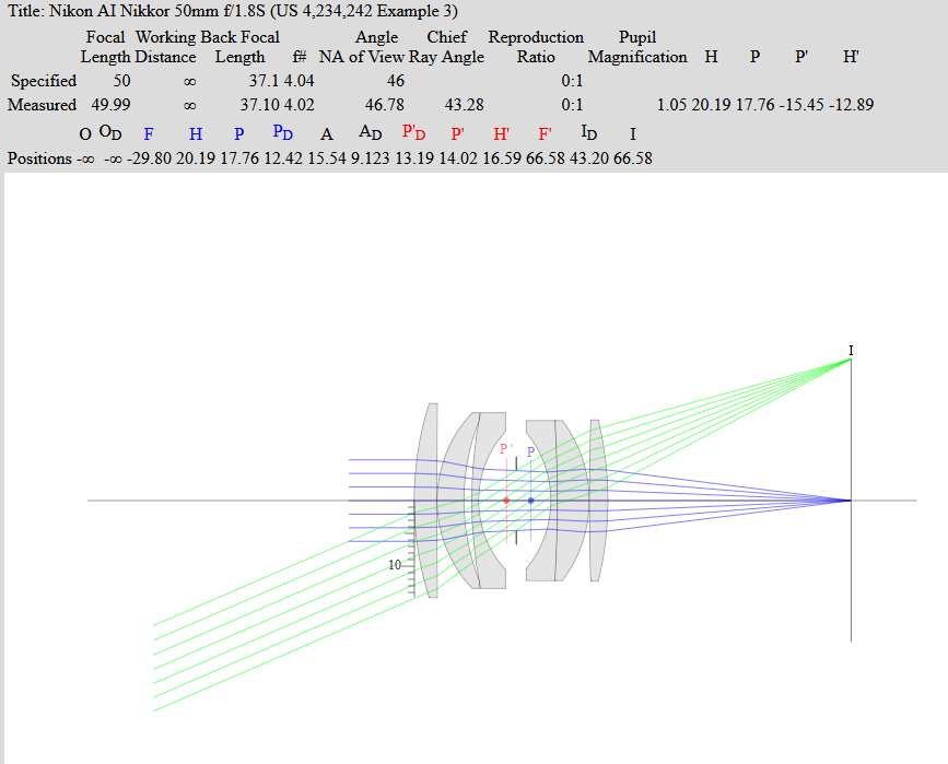
Nikon 50 mm f/1.8 at f/4 - The entrance pupil (Pd in blue) is 12.42 mm.