Measuring the bandpass of a narrow band filter or an etalon with a slit spectrometer
Examples of configurations
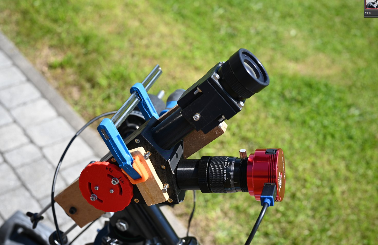
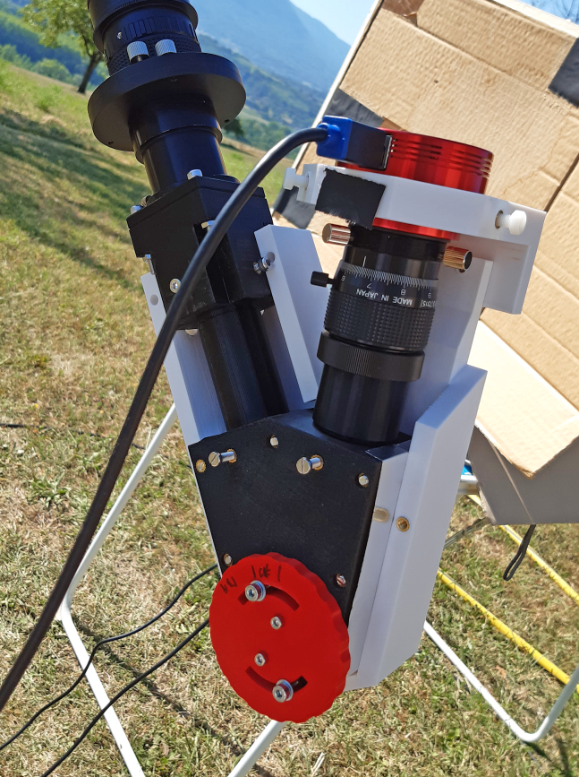
Configuration with 125 mm f.l. collimator, 125 mm f.l. imager and ASI290.
Left: the filter in placed in front of the slit of the spectro. The Sun is the source of light, resulting is a f/115 nearly collimated beam.
Right: the filter is placed in a telecentric beam (f/30) on a Celestron 8. The spectro is mounted on the filter output.
Methodology
The procedure is as follows:
- Take an image of the solar spectrum without the filter to be measured. Image_1 = Solar_Spectrum_Image.- Take an image of the solar spectrum transmitted by. Image_2 = Solar_Spectrum_With_Filter.
The transmission profile of the filter is given by
T (wavelength) = Solar_Spectrum_With_Filter (wavelength) / Solar_Spectrum_Image (wavelength)
The transmission profile is then curve-fit using Fityk with the relevant function (typically Lorenztian function for a single-stack etalon) in order to estimate the FWHM.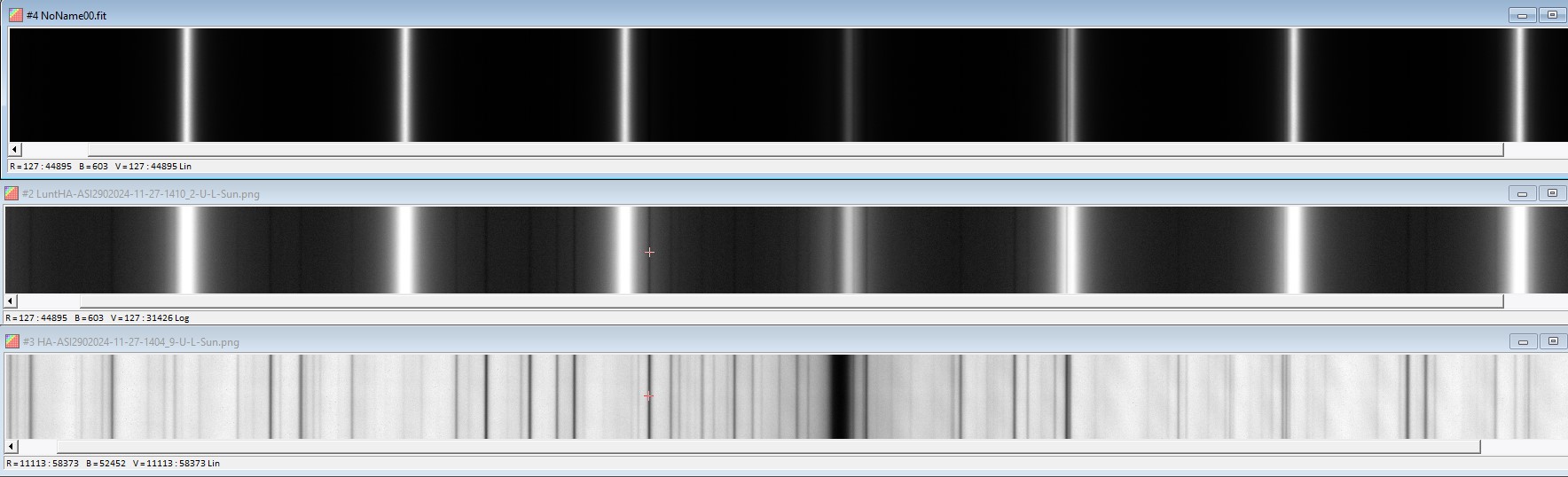
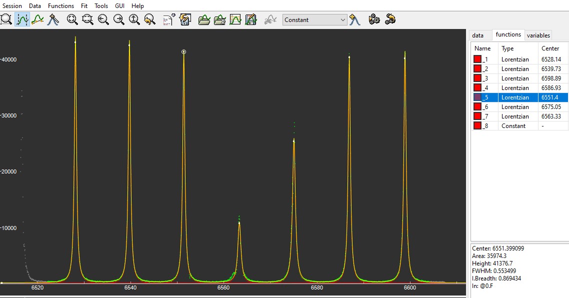
Example 2: measuring a mica-spaced etalon in a telecentric beam
Measuring tips and accuracy of the measurement
Equipement:
- Accurate focusing of both the collimating and the imaging lenses is very important, especially in the near UV (Ca, K, or H). Note that the focus for Ca K is different from the focus for Ca H, which is different from the focus for Ha.
- Diffraction limited collimating and imaging lenses are essential, especially in the near UV where lens spherical aberration is usually very important.
- To maintain accurate focusing throughout the measurement, it is important that the temperature of the spectroscope be as stable as possible. Note that the CTE of aluminum is twice that of PETG.
- It is advantageous to cover the spectroscope with a black shroud to minimize background light. Check light leakage using long exposure times and blocking light on the slit.
- For acquisition :
- use maximum number of bits of the camera,
- use the minimum value gain,
- set the offset so that there is no threshold effect,
- chose an exposure time long enough to fill the histogram up to 80-90%. Note that exposure time can goes up to 1s for very dark mica-spaced etalon.
- choose an acquisition duration long enough to have a good S/N. Typical duration ranges from 10 s (for high transmission air-spaced etalons) to more than 30 s (for low transmission mica-spaced etalons).
- no not change any acqusition parameters when recording the solar spectrum and the spectrum, except the exposure time.
- stack all the frames of the SER file (no registration, no selection of images).
- Non linearity of the sensor can cause some distortion in the estimation of the transmission profile of the filter. The linearity of the sensor can be checked using SharpCap. See some examples here : Sensor linearity
- Tuning etalons :
- It is better to tune etalons away from Ha for the measurement. Indeed, setting the etalon right on Ha can cause distortion effect due to non-linearity of the sensor.
- It is better to measure air-spaced etalons without their Blocking Filters because more fringes can be measured.
Measurement:
- For etalons, the curve fit should be done with a Lorentzian curve (or a Voigt if the etalon is not uniform). A fit with a Gauss function is not accurate enough.
- As a rule of thumb, in order to measure a filter with a bandpass equal to FWHM, the dispersion of the spectroscope should be greater than FWHM/4 (e.g. 0.125 A/pixel dispersion for measuring a 0.6 A etalon). Otherwise, the curve fit will not be accurate enough.
- For the same reason, and more importantly, the spectral resolution (= bandwidth of the spectroscope) should be related to the FWHM of the etalon being measured. A spectral resolution better than FWHM/2 is recommended.
Cross-check results:Note on measuring the dispersion of the spectroscope
To perform the previous measurements, we need to know the dispersion of the spectroscope (A/pixel). It can be measured very easily, without the need of using reference lamps or a specialized software dedicated to spectroscope.
The dispersion of a spectroscope depends on the wavelength. The good news is that we don't need the full relation dispersion = f (wavelength). We only need to know the dispersion around the Ha line (or any other line of interest to measure a narrow band filter).
Two methods can be used :
(1) - Simply use the Simspec.xls spreadsheet provided by Ken Harrison.
The main uncertainty in this approach is that the focal length of the collimating and imaging lenses is known to an accuracy of +/1%for the designed wavelength (for lenses provided by Thorlabs), and changes with wavelength.
Still, resulting accuracy is in the range of +/-5% which is quite reasonable for the use we have.
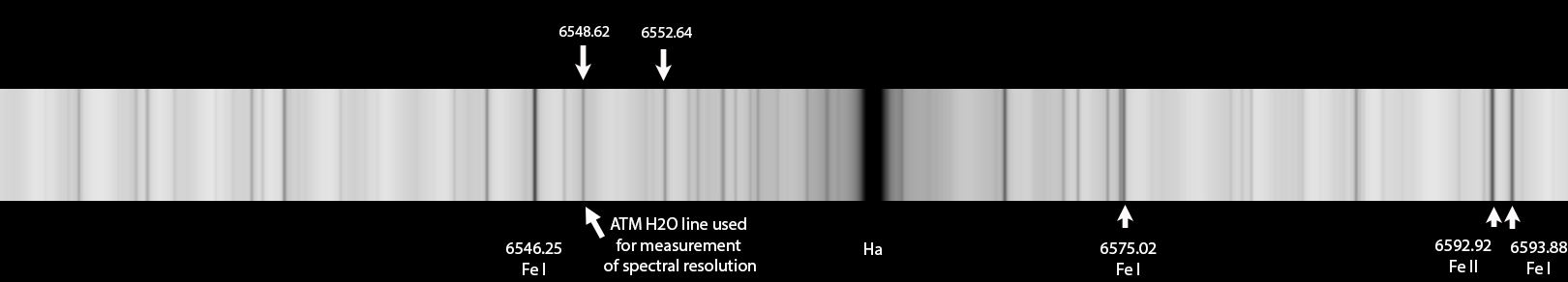
(2) - Actually measure the dispersion around Ha using the solar reference spectrum provided by Bass2000.
https://bass2000.obspm.fr/solar_spect.php
Using this reference very high resolution reference spectrum, the wavelength of the solar lines can be measured to a accuracy of better than 0.01 A, which is much is more than enough. This work has already been done here: